A map shows where things are. The attribute table says what they are. Every polygon, line and point in a vector layer has a row in that table, and almost everything a GIS does beyond drawing pictures happens through it. Styling by category, filtering a layer, calculating a statistic, joining a spreadsheet to a boundary file are all attribute table operations.

This guide covers what the table holds, the limits imposed by the file format, the operations that matter in daily work, and the mistakes that cost the most time.

What an Attribute Table Is

An attribute table is a table in which each row is one feature of a layer and each column is one property of those features. Columns are called fields and rows are called records. A layer of city districts has one row per district, with fields such as name, population and area.

The link between a row and its geometry is maintained by the GIS through an internal identifier, usually called FID or a similar name depending on the format. That identifier is why deleting a row deletes the shape on the map as well, and why a row cannot exist without its geometry in a normal vector layer.

One point is worth clearing up. Raster layers do not have attribute tables in this sense, because a raster stores values in cells rather than features. Categorical rasters can carry a separate value table that describes what each class means, but that is a different structure from a vector attribute table.

Field Types and Why They Matter

Each field has a type, and the type is fixed when the field is created. Choosing the wrong one causes problems that surface much later.

The most common and most expensive mistake is storing identifiers as numbers. Postal codes, district codes and cadastral numbers often begin with a zero, and a numeric field silently removes it. The code 01234 becomes 1234, the join against another dataset fails, and the cause is not obvious. Identifiers belong in text fields even when they look like numbers.

The File Format Decides What the Table Can Hold

Attribute tables are not format independent, and the shapefile is where most surprises happen. It remains the most exchanged vector format, and its attribute component is a dBASE file from the 1980s with the limits to match:

• Field names are truncated to 10 characters, so building_height and building_heating become the same field name.

• A maximum of 255 fields per layer.

• Text fields hold at most 254 characters.

• Both the .shp and the .dbf are capped at 2 GB.

• Dates are stored without a time component.

• Unicode support is weak, so names in non Latin alphabets need a matching .cpg encoding file or they arrive as unreadable characters.

• There is no reliable NULL, so an empty numeric cell often reads back as zero, which is a real value and not an absence of one.

GeoPackage avoids all of these. It is a single SQLite file with full length field names, proper date and time types, real NULL support and no practical size ceiling, and it is an OGC standard. PostGIS goes further for multi user editing. GeoJSON is convenient for exchange and the web, and it has no schema enforcement at all, which means a field can hold a number in one feature and text in the next.

The practical rule is to keep working data in GeoPackage or PostGIS and treat the shapefile as an exchange format, checking field names after every export to it.

Selecting and Filtering by Attribute

These two operations look similar and behave differently, which is a frequent source of confusion. A selection marks records while leaving the whole layer visible. A filter hides everything that does not match, so the hidden records are excluded from the map, from the table and often from subsequent processing.

Both are driven by expressions. The syntax follows SQL closely across GIS tools, and the useful building blocks are few:

• Comparison with equals, greater than, less than, and not equal.

• Combination with AND, OR and NOT, with brackets to control the order.

• Partial text matching with LIKE and a wildcard, for example name LIKE 'North%'.

• Membership with IN, for example type IN ('school', 'clinic').

• Emptiness with IS NULL and IS NOT NULL, which is not the same as equalling zero or an empty string.

The distinction between NULL, zero and an empty string catches people constantly. A population field holding 0 means nobody lives there. The same field holding NULL means nobody measured it. A query that treats them alike will produce a confident wrong answer.

Calculating Fields

A field calculator writes values into a field using an expression, either into a new field or over an existing one. Typical uses are computing area and length from geometry, deriving a density from two existing fields, building a label by concatenating text, and reclassifying values into categories.

One trap deserves its own warning. Calculating area or length while the layer is in a geographic coordinate system such as WGS 84 produces a result in square degrees, which is not a unit of area and varies with latitude. The number looks plausible and is meaningless. Area and length calculations belong in a projected coordinate system chosen for the region, and the result should always be sanity checked against a known object.

Calculations that overwrite an existing field are usually not undoable after saving, so the safe habit is to calculate into a new field and delete the old one once the result has been checked.

Joining Tables

A join attaches a second table to the attribute table using a shared field, which is how statistics from a spreadsheet end up on a map of administrative boundaries. The shared field is the join key, and it has to match exactly on both sides.

Most failed joins come from the key rather than the method:

• Type mismatch, where the key is text in one table and a number in the other.

• Leading zeros stripped by a numeric field, so 01234 no longer matches 01234 stored as text.

• Trailing spaces, which are invisible in the table view and fatal to the match.

• Different spellings of the same name, which is why joining on codes beats joining on names.

Cardinality matters too. A one to one join adds columns and nothing else. A one to many join duplicates geometry or silently keeps only the first match depending on the tool, so a layer that suddenly has more rows than it has features usually has a cardinality problem.

A spatial join works differently, matching records by location rather than by a shared value, which answers questions such as which district each incident falls inside. It needs no common field and depends entirely on both layers being in compatible coordinate systems.

In most desktop GIS a join is virtual, meaning the joined columns exist only while the project is open. Exporting the layer to a new file is what makes them permanent.

Working With the Attribute Table in GISCARTA

In GISCARTA the attribute table is a widget, so it is switched on for a project and then opened per layer.

Opening the table

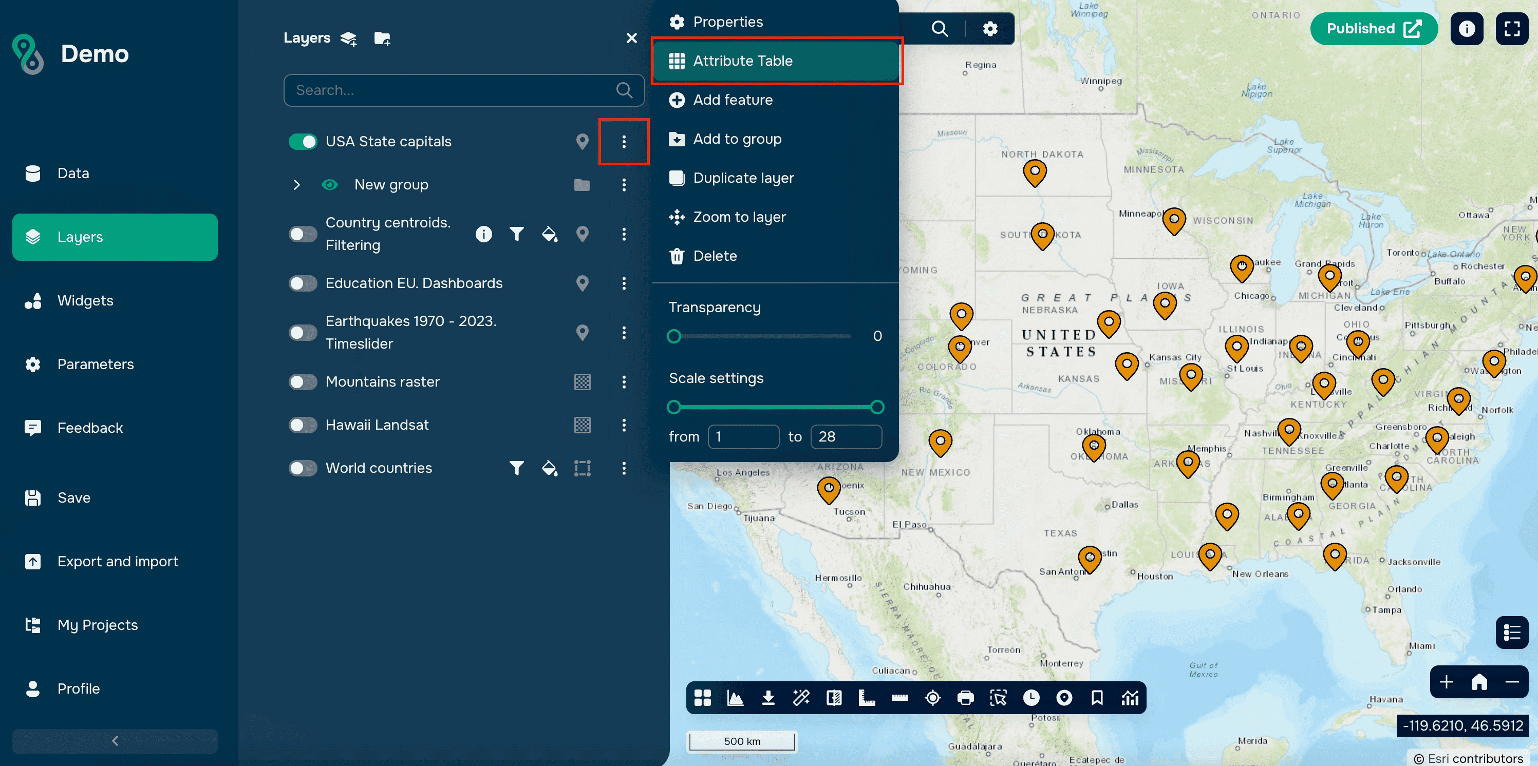
Enable the attribute table in the Widgets section of the project, then open the layer settings through the three dot menu next to the layer and choose the attribute table.

Filtering

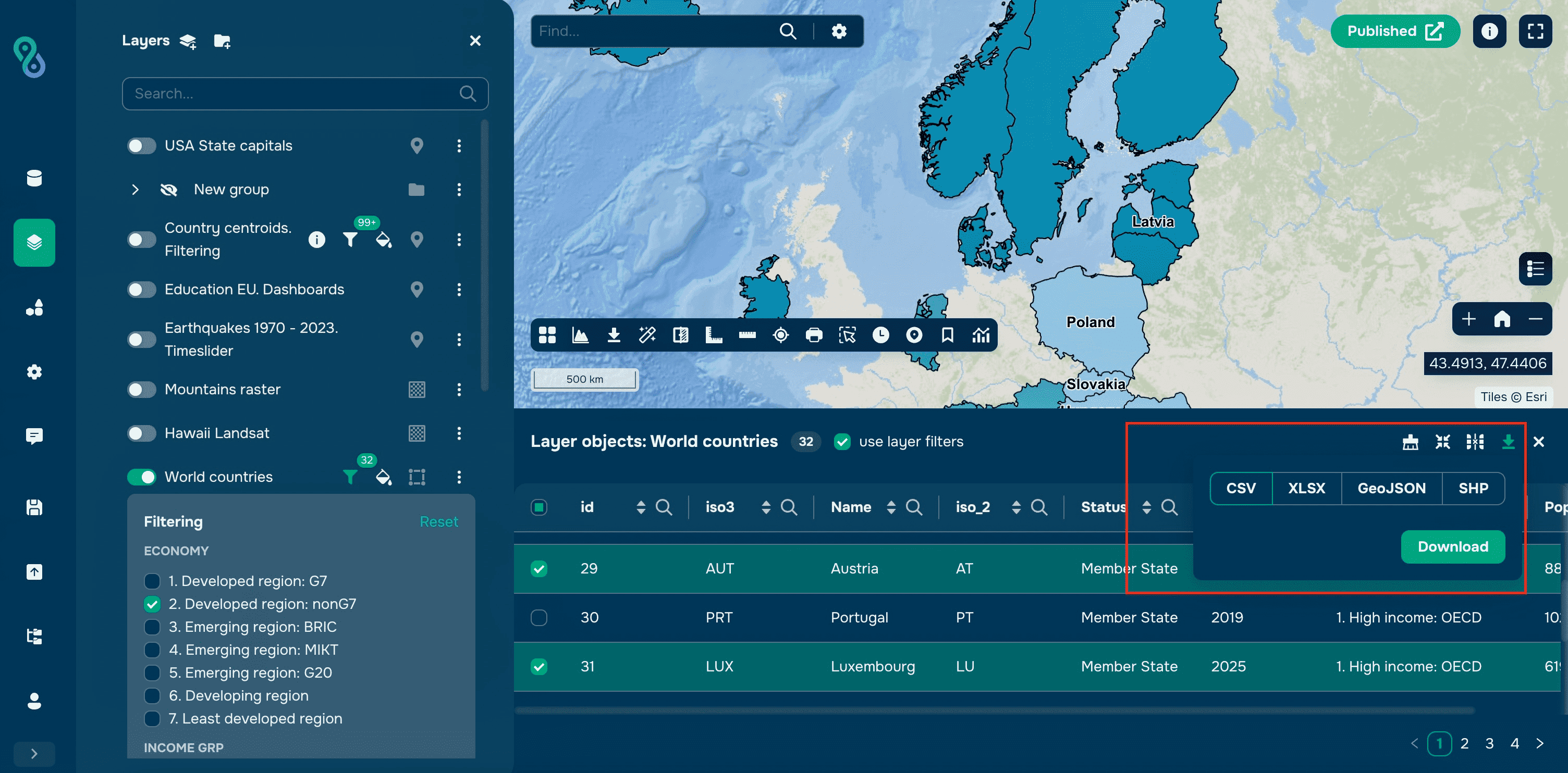
Apply Filter restricts the table to records matching a condition, which is the fastest way to work with a subset of a large layer.

Searching within a column

The magnifying glass searches inside a chosen column, which suits finding a known name or code without writing a condition.

Sorting

The arrows in a column header sort ascending or descending. Sorting a text field that contains numbers gives alphabetical order, which is the behaviour described in the field types section above.

Zooming to selected features

Selecting rows and zooming to them moves the map to those features, which is the quickest way to check that a query returned what was intended.

Hiding columns

Hiding columns affects the view only and leaves the data untouched, which keeps wide tables readable.

Exporting a selection

Selected features export to CSV, XLSX, GeoJSON or SHP. CSV and XLSX carry the attributes alone, while GeoJSON and SHP carry geometry with them, and the shapefile limits described earlier apply to that last option.

Common Mistakes

• Storing codes and identifiers in numeric fields, which strips leading zeros and breaks joins later.

• Treating NULL and zero as the same value in queries and statistics.

• Calculating area or length in a geographic coordinate system and reporting square degrees as if they were square metres.

• Exporting to shapefile without checking the truncated field names afterwards.

• Joining on names instead of codes, which fails on spelling and spacing differences.

• Editing attributes without a copy of the original file, since most attribute edits cannot be undone after saving.

• Forgetting that a join is virtual until the layer is exported.

FAQs

What is the difference between a field and a record?

A field is a column describing one property across all features. A record is a row holding every property of a single feature.

Why did my field names change after saving to shapefile?

The shapefile format truncates field names to 10 characters. Names that share their first 10 characters collide and receive numeric suffixes. Saving to GeoPackage instead avoids the problem entirely.

Why do my area values look wrong?

Almost always because the layer is in a geographic coordinate system, so the calculation returns square degrees. Reproject to a projected system appropriate for the region and calculate again.

Why does my join return empty columns?

The join keys do not match exactly. Check that both are the same type, that no leading zeros have been stripped and that neither side has trailing spaces.

Can an attribute table exist without geometry?

Yes. Standalone tables such as CSV or spreadsheet files are common in GIS projects and are used precisely so that they can be joined to a spatial layer later.

Key Takeaways

The attribute table is where most GIS work actually happens, because styling, filtering, analysis and joins all read from it.

Field types and the file format set hard limits on what can be stored, and the shapefile is the most restrictive of the common formats.

Most lost time comes from a small set of predictable errors, above all mismatched join keys, confusion between NULL and zero, and area calculated in degrees.