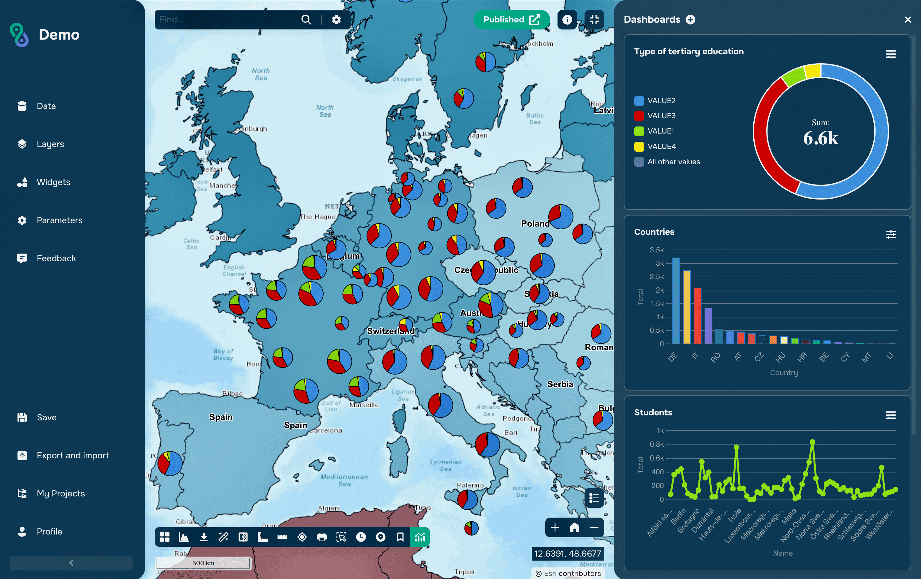
A join brings together data that lives in different tables. In GIS there are two ways to decide which records belong together: matching a shared value, or matching position on the map. The first is an attribute join, the second a spatial join. They solve different problems, fail in different ways, and mixing them up is one of the most common sources of wrong numbers in a report.
Spatial Join vs Attribute Join: What Is the Difference?
An attribute join needs a key: a field that exists in both datasets and holds the same values, such as a municipality code or a parcel number. A spatial join needs no key at all, because the relationship is derived from geometry: which points fall inside which polygon, which lines cross which boundary, which facility is nearest.

How Spatial and Attribute Joins Differ
Spatial Join vs Attribute Join
Feature | Attribute join | Spatial join |
Basis of matching | Equal values in a common field | Spatial relationship between geometries |
Common key required | Yes | No |
Same coordinate system required | No | Yes, otherwise reprojection first |
Typical inputs | Layer and a table | Two layers with geometry |
Result | Attributes added by key value | Attributes added by location |
Cardinality | Usually one to one or one to many | Often one to many, needs aggregation |
Determinism | Exact value comparison | Depends on geometry and tolerance |
Index used | Attribute index | Spatial index |
Computational cost | Low | Higher, geometry is compared |
In SQL | JOIN ON a.code = b.code | JOIN ON ST_Intersects(a.geom, b.geom) |
Typical use | Statistics by code, lookup tables | Points in polygons, nearest object, overlay |
Typical failure | Keys that look equal but are not | Wrong relationship or mismatched CRS |
What Is an Attribute Join?
An attribute join attaches a table to a layer through a shared field. The classic case is a boundary layer of districts and a spreadsheet of population figures: both carry an official district code, so the statistics can be mapped without touching geometry at all.
Because the operation is a value comparison, it is fast and completely predictable. It also makes no claim about space: if the codes are wrong, the join will still succeed and silently attach the wrong numbers to the wrong polygons, which is why the count of matched records should always be checked against the number expected.
What Is a Spatial Join?
A spatial join transfers attributes based on how geometries relate. Typical questions it answers are which district each incident belongs to, how many customers fall within a service area, which road segment is nearest to each address, or what land-cover class underlies each sample point.
It is the tool of choice when no shared identifier exists, which is common when data comes from different organizations. The price is that the result depends on two things an attribute join never involves: the coordinate system of both layers, and the exact geometry near boundaries.
Spatial Relationships
The relationship chosen defines the result. Intersects is the broadest and includes any contact, including a point lying exactly on a boundary. Within and contains require full containment, so a polygon that sticks out even slightly is excluded. Touches matches only shared boundaries without shared interiors, and crosses applies to lines passing through an area.
Two further options are worth knowing because they answer questions the topological predicates cannot. Nearest, called closest match in ArcGIS Pro and available in QGIS as a separate tool, links each object to the closest one, and within a distance uses a threshold, which is how the notion of an object near but not inside a boundary is expressed.
One Match or Many
A spatial join usually produces more than one match. A district contains hundreds of incidents, and a parcel may intersect several soil polygons, so the software offers a choice: keep one record per source object with a summary, or produce one record per matched pair.
Summarizing is where the analytical decision lives. Counting incidents per district is straightforward, but averaging a value across overlapping polygons of unequal size is not, and area-weighted values usually require intersecting the layers first and computing the weights explicitly. When a report shows suspiciously round or identical numbers across districts, an unweighted average from a spatial join is a frequent explanation.
Attribute joins have the same issue in a quieter form. Joining a table that contains several rows per key multiplies the features, so a layer of 100 districts can silently become 340 records, and every subsequent sum is inflated.
Performance and Indexes
Both operations depend on indexes, but different ones. An attribute join uses an index on the key field; a spatial join uses a spatial index, which first compares bounding boxes and only then runs the exact geometry test on the few candidates that remain.
This is why a spatial join that takes seconds in PostGIS can take many minutes on the same data in a file-based format without an index. Two more factors matter: complex polygons with thousands of vertices cost far more to test than simple ones, so simplifying boundaries that are more detailed than the task requires can change runtime by an order of magnitude, and layers in different coordinate systems must be reprojected before the join rather than relying on on-the-fly display.
Where Joins Fail
Attribute joins fail on keys that look identical on screen. A code stored as text in one table and as a number in another will not match, leading zeros disappear when a code passes through a spreadsheet, and trailing spaces, differing letter case and mismatched encodings all break equality. Trimming, padding and casting the key to a single type before joining removes most of these cases.
Spatial joins fail at boundaries. A point that falls exactly on a shared edge intersects both adjacent polygons and is counted twice, sliver polygons from slightly different digitizing of the same border produce spurious matches, and coordinates rounded during export can move an object across a line. Choosing a stricter relationship, or snapping and cleaning the geometry first, is usually more reliable than adjusting tolerances afterwards.
In Practice
QGIS separates the two explicitly: Join attributes by field value for keys and Join attributes by location for geometry, both available as processing tools that write a new layer. The layer properties dialog also offers a temporary join that exists only in the project, which is convenient for viewing but is a frequent surprise when the file is opened elsewhere and the fields are gone.
ArcGIS Pro offers Add Join for a temporary attribute join, Join Field to write the values permanently, and Spatial Join for geometry, with match options and field mapping that control how multiple matches are summarized. In SQL both are the same statement with a different condition, and in PostGIS a spatial join is an ordinary JOIN whose ON clause calls ST_Intersects, ST_Within or ST_DWithin.
Common Mistakes
The most common mistake is not checking how many records matched. Both join types report it, and comparing that number with the expected count catches key mismatches, duplicated rows and empty results before they reach a map.
The second is using a spatial join where a key already exists. If both datasets carry the same official code, matching on it is faster, exact and reproducible, while a spatial join introduces boundary effects for no benefit.
The third is treating the joined result as permanent. Temporary joins live in the project, not in the data, so results that will be shared, analyzed further or opened by someone else should be written to a new layer or field.
FAQs
Which join should be used when both are possible?
The attribute join, provided the key is reliable. It is faster, exact, and unaffected by geometry quality or coordinate systems.
Why are some features missing after a spatial join?
Usually because the join kept only matched records, the relationship was stricter than intended, or the layers were in different coordinate systems. Running the join with a retain-all-features option shows immediately which objects found no match.
How is a point on a boundary handled?
With an intersects relationship it belongs to every polygon it touches, so it appears more than once. Deciding the rule in advance, for example by assigning such points to a single polygon by an additional criterion, prevents double counting.
Can a join produce more rows than the original layer?
Yes, in both cases. A one-to-many relationship duplicates each source feature once per match, which is correct behaviour but makes any subsequent sum wrong unless the duplication is intended.
Is a spatial join the same as an overlay?
No. A spatial join transfers attributes and leaves the geometry of the target layer unchanged, while an overlay such as intersect or union creates new geometry from the inputs. When area-weighted values are needed, the overlay is the correct starting point.
Key Takeaways
The two joins answer different questions. An attribute join asks which records share an identifier and gives an exact, cheap and reproducible answer whenever a reliable key exists. A spatial join asks which records share a location and makes it possible to combine data that was never designed to be combined, at the cost of sensitivity to coordinate systems, geometry quality and the choice of relationship.
In a well-organized workflow the two are used in sequence: a spatial join establishes the link once, the resulting identifier is written into the data, and everything afterwards runs on attribute joins. That turns a fragile geometric operation into a stable key and makes the results reproducible by anyone who repeats the analysis.